Surface Oversampling#
Dependencies#
[2]:
%load_ext autoreload
%autoreload 2

from cryocat.core import cryomap
from cryocat.analysis import surfsamp
from cryocat.core import cryomotl
import numpy as np
import pandas as pd
import os
from skimage.transform import resize
Expected time#
All steps should be completed within seconds/minutes. The boundary_sampling and inner_and_outer_pc might took longer depend on the amount of points.
Input data#
Loading shape labels and sampling the surface#
[3]:
spcsv = surfsamp.SamplePoints.load("inputs/040_1_shape.csv")
spcsv.boundary_sampling(sampling_distance = 10)
Loading mask and sampling the surface#
[4]:
spmask = surfsamp.SamplePoints.load("masks/040_generated_mask_2.mrc")
spmask.boundary_sampling(sampling_distance = 10)
Writing the sampling points into motl_list.em file#
[ ]:
tomo_id = '040'
obj_id = '001'
input_dict = {'tomo_id':np.ones(spmask.vertices.shape[0])*float(tomo_id), 'object_id':np.ones(spmask.vertices.shape[0])*float(obj_id)}
spmask.write("expected_outputs/motl_040mask_sp10.em", input_dict)
spcsv.write("expected_outputs/motl_040csv_sp10.em")
Reset normal of points#
The point cloud generated by boundary_sampling can also be used to replace the normals in a motl_list. The normal of the nearest point to each motl point will be used to update its angle.
[ ]:
# parameters for making the oversample points in right binning
b_factor = 4
pal_thickness = 20
samp_dist = 10

mask = cryomap.read("040_generated_mask_2.mrc")
# bin mask base on b_factor
size = tuple(b_factor*i for i in mask.shape)
bin_mask = resize(mask, size, order=0, mode='constant')
# generate oversample points using bin mask
spmask40 = surfsamp.SamplePoints.load(bin_mask)
spmask40.boundary_sampling(sampling_distance = samp_dist)
spmask40out,_ = spmask40.inner_and_outer_pc(thickness = pal_thickness*b_factor)
# load motl which you want to modified
motl = cryomotl.Motl.load('inputs/motl_040_STAexample.em')
spmask40out.reset_normals(motl)
motl.write_out('expected_outputs/motl_040_STArenormal.em')
Calculate surface area#
[ ]:
# You may notice that spmask has twice the area of spcsv.
# This is because the mask input represents a shell, whereas spcsv only considers the outer surface.
print(spmask.area)
print(spcsv.area)
Oversampling the mask surface and generating a motl_list for multiple tomograms.#
[ ]:
# Sampling and create point clouds base on the surface of the mask. Keep only the outer shell of the pointcloud and save into a motl_list
mask_folder = f'masks'
mask_list = f'inputs/mask_list.csv'
output_folder = f'expected_outputs/motls'
pal_thickness = 20
sampling_dist = 5
shift_dist = -6

# read in mask_list
mask_array = pd.read_csv(mask_list, header=None).to_numpy().astype(str)
# zero-padded tomo number to 3 digits
mask_array[:, 0] = np.char.zfill(mask_array[:, 0], 3)
for i in mask_array:
    tomo_id, obj_id = i
    # file name of input and output
    mask_file = f'{tomo_id}_generated_mask_{obj_id}.mrc'
    motl_file = f'{tomo_id}_{obj_id}_pointcloud.em'
    mask = cryomap.read(f'{mask_folder}/{mask_file}')
    # sampling at the surface of mask and keeping only the outer sample points of the shell
    sp = surfsamp.SamplePoints.load(mask)
    sp.boundary_sampling(sampling_distance = sampling_dist)
    outer_sp,_ = sp.inner_and_outer_pc(thickness = pal_thickness)
    # shifting coordinates 6 pixels in opposite normal vectors direction. negative value for shifting into direction opposite of the normal vectors
    outer_sp.shift_points(shift_dist)
    # create input_dict to fill in 'tomo_id' and 'object_id'
    input_dict = {'tomo_id':np.ones(outer_sp.vertices.shape[0])*float(tomo_id), 'object_id':np.ones(outer_sp.vertices.shape[0])*float(obj_id)}
    outer_sp.write(f'{output_folder}/{motl_file}', input_dict)
    print(f'{motl_file} was written')
In case you would like to shift different distance for different normals use method shift_points_in_groups with shift_dict input. The shift_dict is a dictionary where keys are tuples representing normal vectors and values are the shift magnitudes in pixels. Here’s an example of shifting points with normals pointing out/into the tomogram with a distance in 20 pixels and others in -6 pixels
[ ]:
shift_dist = -6
shift_dist_tb = 10
# To create a shift_dict with keys from all normal vectors
shift_dict = {key: shift_dist for key in tuple(map(tuple,outer_sp.normals))}
# assgin different value for target normal vectors
shift_dict[(1,0,0)] = shift_dist_tb
shift_dict[(-1,0,0)] = shift_dist_tb
# run shift_points_in_groups
outer_sp.shift_points_in_groups(shift_dict)
Merging and renumbering all motls from each object into one
[ ]:
motl_name = sorted(os.listdir(output_folder))
motl_merge = cryomotl.Motl.merge_and_renumber([f'{output_folder}/{i}' for i in motl_name])
motl_merge.write_out(f'expected_outputs/allmotl_pcShift-6.em')
Contours and mask on Napari#
Dependencies#
Napari should be installed on extra:
pip install napari
[ ]:
%load_ext autoreload
%autoreload 2

import napari
import numpy as np
import pandas as pd
from cryocat.core import cryomap
from cryocat.analysis import surfsamp
Input data#
The data for this tutorial can be downloaded here.
There’s no expected output for this tutorial since the drawing is user-generated. However, you can refer to ‘inputs/040_1_shape.csv’ as an example shape from us for this tomogram and ‘inputs/masks/040_generated_mask2.mrc’ on owncloud as an example mask.
Initialize the napari viewer and load tomogram#
[ ]:
#Initialize the napari viewer:
view = napari.Viewer()
# Load tomogram from owncloud and add it to the viewer
tomo = cryomap.read('040.mrc')
view.add_image(tomo)
Contours in Napari#
Draw contour on Napari#
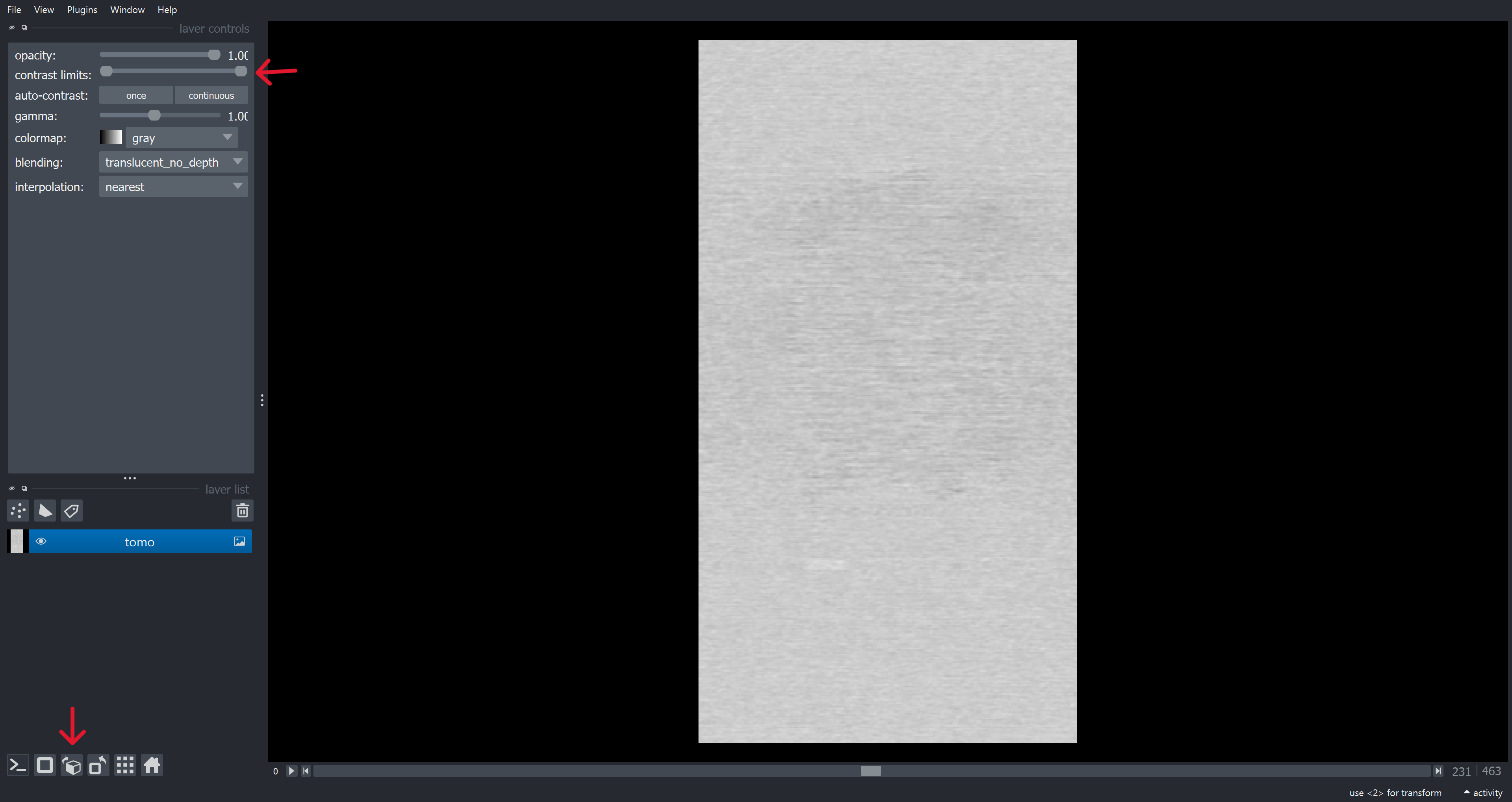
In the Napari GUI, click the small cube button at the bottom left of the screen to change the order of the visible axes. You can also adjust the visualization contrast using the contrast limit.
Create a new shape layer using the polygon button located in the middle left. Then, draw the contour using the “Add Polygons” button. Drawing contours on multiple axes can improve the accuracy of sampling points on the target surfaces. For a detailed guide on using shape layer, refer to page here

Save shapes into CSV#
Once you’ve finished drawing, you can save your shapes to a CSV file by running the following code. The CSV file can later be loaded into Napari for modifications and visualization.
[ ]:
def save_shapes(shape_layer, output_file_name):
    """This function saves the shape layer data into a csv file.

    Parameters
    ----------
    shape_layer : list
        A list of numpy arrays where each array represents a shape layer. Each array is expected to have three columns representing the x, y, and z coordinates respectively.
    output_file_name : str
        The name of the output file where the shape layer data will be saved.

    Returns
    -------
    None

    Notes
    -----
    The function creates a pandas DataFrame from the shape layer data and saves it into a csv file. The DataFrame has four columns: 's_id', 'x', 'y', and 'z'. The 's_id' column represents the shape layer id, 'x', 'y', and 'z' columns represent the coordinates of the shape layer.
    """
    x = []
    y = []
    z = []
    s_id = []

    for i in range(len(shape_layer)):
        x.append(shape_layer[i][:, 2])
        y.append(shape_layer[i][:, 1])
        z.append(shape_layer[i][:, 0])
        s_id.append(np.full(shape_layer[i].shape[0], i))

    x = np.concatenate(x, axis=0)
    y = np.concatenate(y, axis=0)
    z = np.concatenate(z, axis=0)
    s_id = np.concatenate(s_id, axis=0)

    # dictionary of lists
    dict = {"s_id": s_id, "x": x, "y": y, "z": z}

    df = pd.DataFrame(dict)
    # saving the dataframe
    df.to_csv(output_file_name, index=False)


# output file name
output = 'inputs/040_1_shape_fromUser.csv'
# saving shapes for future work
shapes_data=view.layers[1].data
save_shapes(shapes_data, output)
Read and view shape CSV on napari#
[ ]:
# opening the shape layer which is provided in inputs folder
polygons = surfsamp.SamplePoints.load_shapes('inputs/040_1_shape.csv')
shapes_layer = view.add_shapes(polygons, shape_type='polygon')
Masks in Napari#
Draw binary segmentation on napari#
Manually drawing a binary mask can be time-consuming. Depending on your dataset, a more efficient solution may be available. Such as using MemBrain-Seg for membrane segmentation in 3D for cryo-ET.
[ ]:
# create a empty label
label = np.zeros(tomo.shape, dtype=int)
# add label to the viewer
view.add_labels(label)
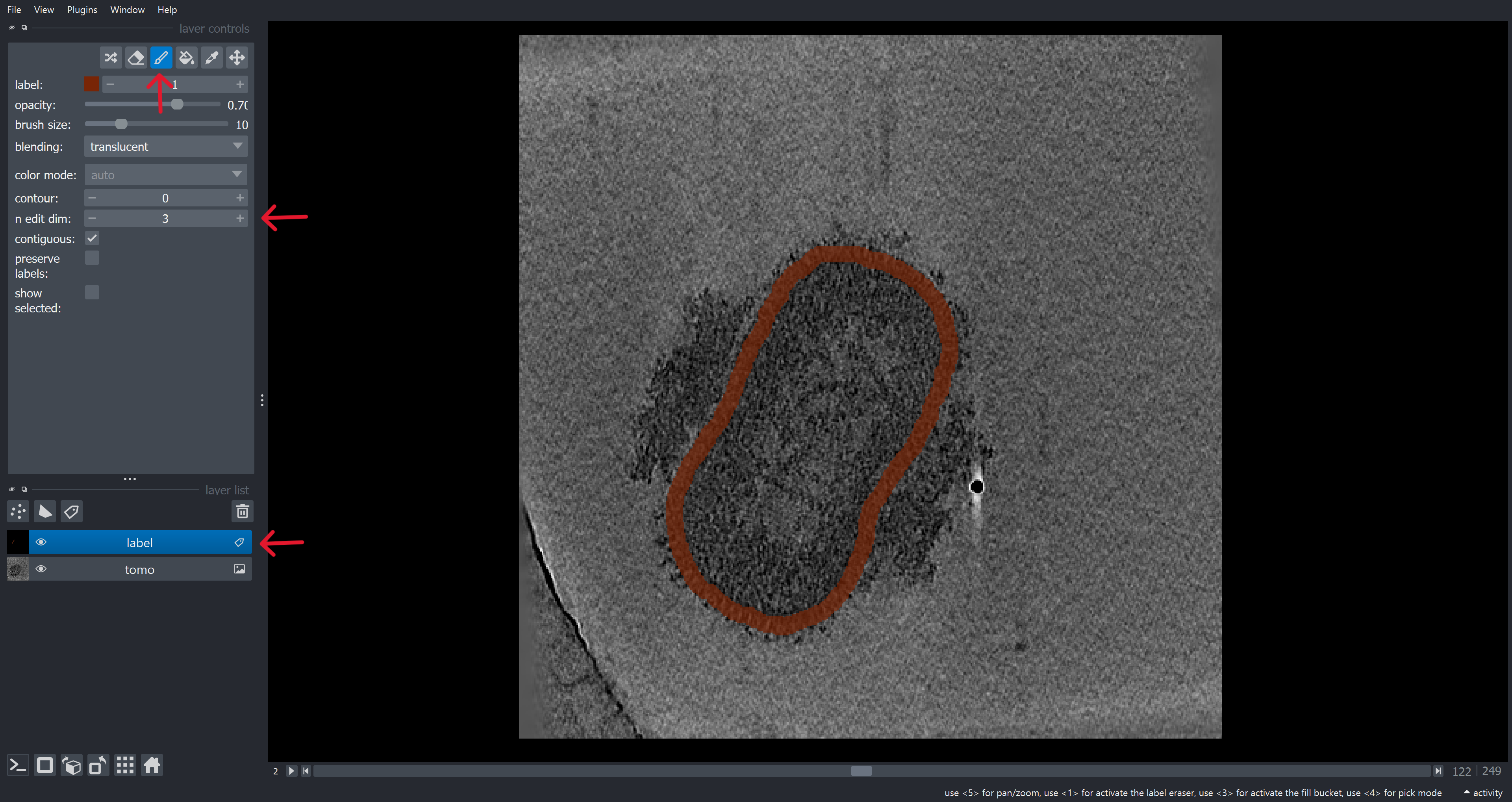
In the Napari GUI, select the label layer and choose the brush tool at the top. You can draw the mask by left-clicking and dragging your mouse. To draw in 3D, set ‘n edit dim’ to 3. To label multiple objects on same tomogram, assign a different number to each label before drawing. For more information of how to use label in napari, refer to page here
Save binary segmentation into mrc#
Once you’ve finished drawing, you can save your labels as an MRC file using the following code. The MRC file can later be opened in Napari for further analysis.
[ ]:
# output file path
output = 'inputs/040_mask_fromUser.mrc'
# saving label for future work
label = view.layers[1].data
cryomap.write(label, output, data_type='<f4')
Simple postprocess of binary segmentation#
In surfsamp, process_mask can perform simple morphological operations on a given mask. It can also be used for manually drawn masks to refine or modify them as needed. There are four available options: ‘closing,’ ‘opening,’ ‘dilation,’ and ‘erosion.’
[ ]:
# for example to dilate the mask for 2 pixels
dil_label = surfsamp.SamplePoints.process_mask(label,2,'dilation',data_type='int')
view.add_labels(dil_label)
Read and view mask as label on napari#
[ ]:
# opening the mask downloaded from owncloud
input = '040_generated_mask_2.mrc'
mask = cryomap.read(input, data_type='int')
view.add_labels(mask)